Colors & Palettes

Complete guide to the CPAL color system

Consistent color usage is essential for creating professional, recognizable data visualizations. The cpaltemplates color system provides 25 functions for working with CPAL’s carefully designed color palettes in R and ggplot2. All colors are sourced from _brand.yml and designed for WCAG accessibility compliance, ensuring your charts are readable by users with color vision deficiencies.

Whether you’re creating a quick exploratory plot or a polished visualization for a report, these functions make it easy to apply CPAL branding consistently across all your R-based data products.

---

Primary Brand Colors

CPAL’s 6 core brand colors form the foundation of all palettes. These colors were carefully selected for brand recognition, accessibility, and versatility across different visualization types.

cpal_colors_primary()

Color	Hex Code	Use Case
Midnight	#004855	Dark backgrounds, headers, primary emphasis
Deep Teal	#006878	Primary brand color, links, info states
Coral	#E86A50	Accents, alerts, negative/error states
Sage	#5A8A6F	Success states, positive indicators
Slate	#5C6B73	Secondary text, borders, muted elements
Warm Gray	#9BA8AB	Neutral backgrounds, disabled states

---

Core Color Functions

These functions are your primary tools for accessing CPAL colors in R. Use them to retrieve color values for ggplot2 visualizations, Shiny apps, or any R-based graphics.

cpal_colors()

The main entry point for accessing any CPAL color or palette. This versatile function handles single colors, multiple colors, and complete palettes—making it the go-to choice for most color needs.

Get all primary colors

cpal_colors()

midnight

#004855

deep_teal

#006878

coral

#E86A50

sage

#5A8A6F

slate

#5C6B73

warm_gray

#9BA8AB

Get a single color by name

cpal_colors("coral")

coral

#E86A50

Get multiple specific colors

cpal_colors(c("midnight", "coral", "sage"))

midnight

#004855

coral

#E86A50

sage

#5A8A6F

Get a palette

cpal_colors("midnight_seq_5")

#E8F4F6

#88BECA

#28889E

#006D88

#004855

Limit number of colors

cpal_colors("main", n = 3)

#004855

#E86A50

#5A8A6F

Reverse palette order

cpal_colors("midnight_seq_5", reverse = TRUE)

#004855

#006D88

#28889E

#88BECA

#E8F4F6

---

cpal_colors_extended()

Returns all 17+ colors including primary colors and shades. Useful when you need access to the full color palette for complex visualizations or custom color schemes.

cpal_colors_extended()

midnight

#004855

deep_teal

#006878

coral

#E86A50

sage

#5A8A6F

slate

#5C6B73

warm_gray

#9BA8AB

teal

#007A8C

gold

#B8860B

plum

#8B5E83

coral_dark

#C75540

neutral

#E8ECEE

midnight_1

#E8F4F6

midnight_2

#B8D9E0

midnight_3

#88BECA

midnight_4

#58A3B4

midnight_5

#28889E

midnight_6

#006D88

midnight_7

#004855

midnight_8

#002D38

success

#5A8A6F

warning

#D4A84B

error

#C75540

info

#006878

---

Viewing Palettes

Before choosing colors for your visualization, it helps to see what’s available. These functions let you explore and preview all CPAL palettes directly in R.

All Available Palettes

list_cpal_palettes()

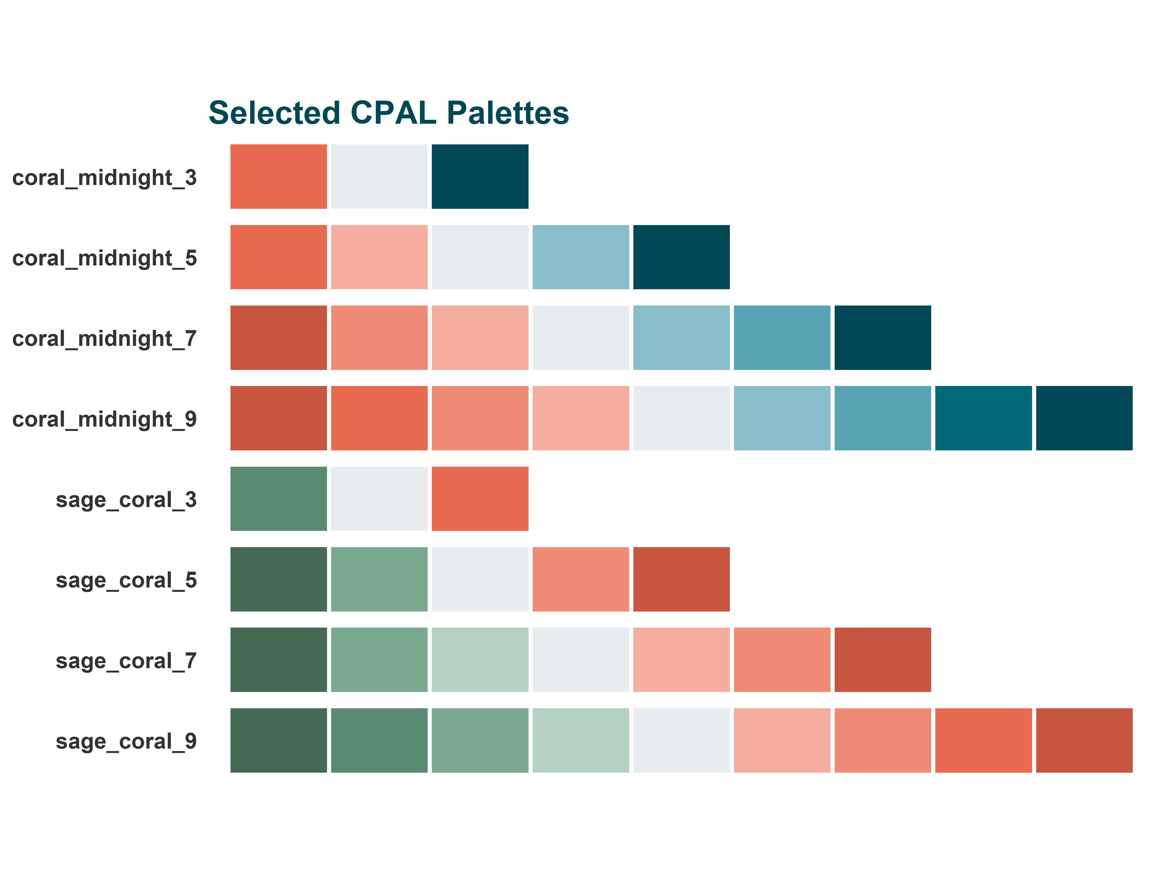
Visual Palette Display

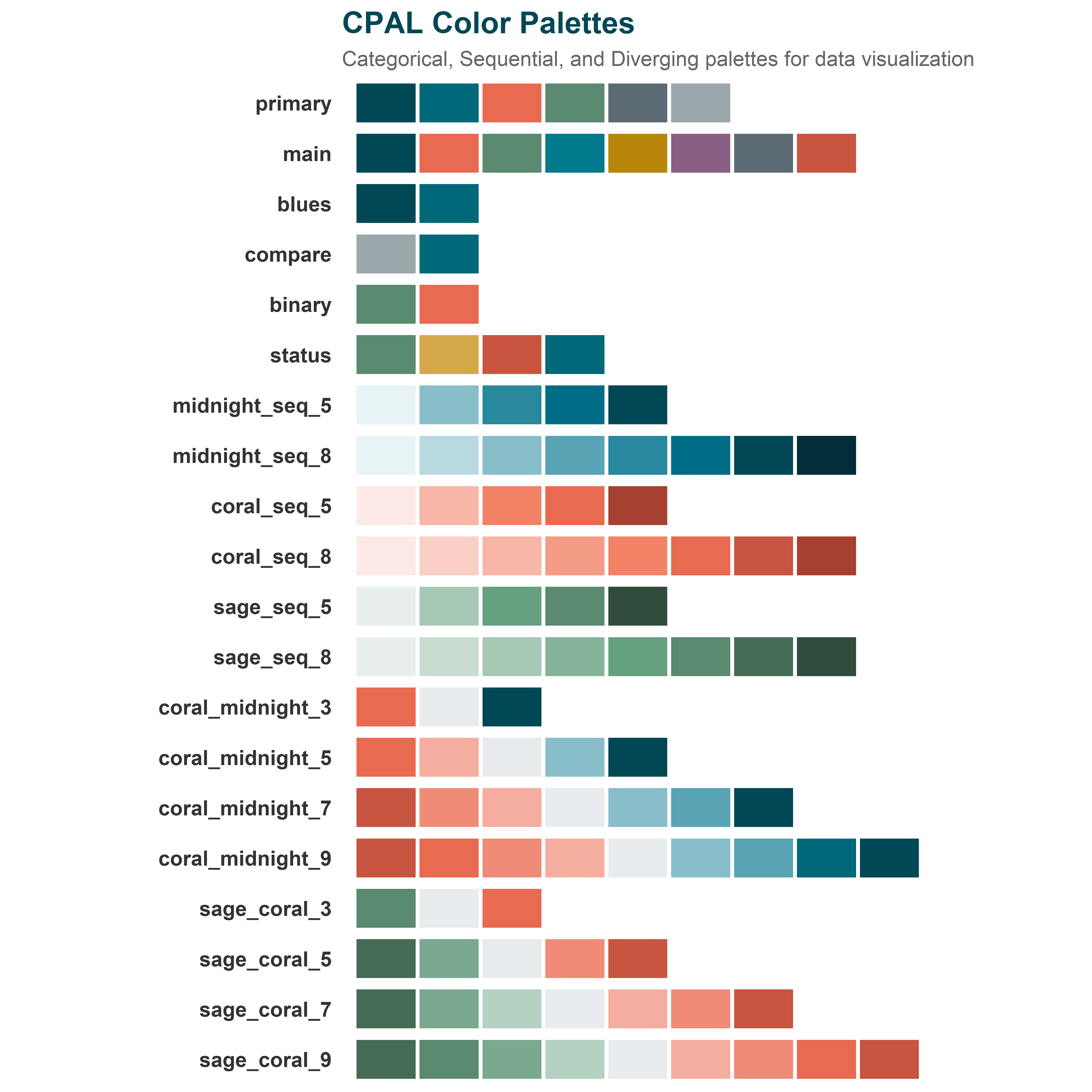
view_cpal_palettes()

All CPAL color palettes

---

Palette Types

Choosing the right palette type is crucial for effective data visualization. Different data types require different color approaches—using a sequential palette for categorical data (or vice versa) can mislead readers or obscure patterns in your data.

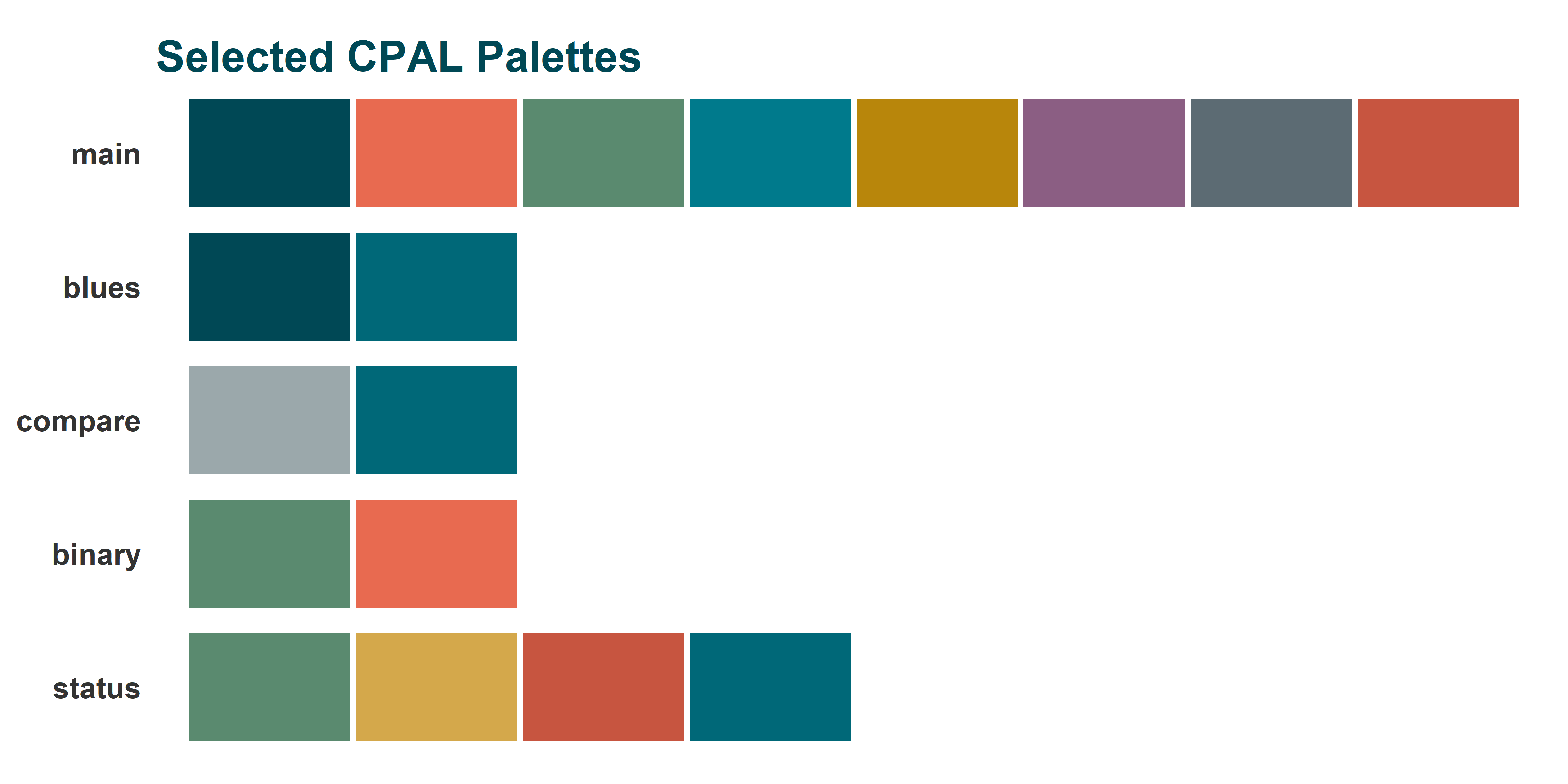
Categorical Palettes

Use for: Discrete data with distinct, unordered categories (e.g., regions, product types, demographic groups).

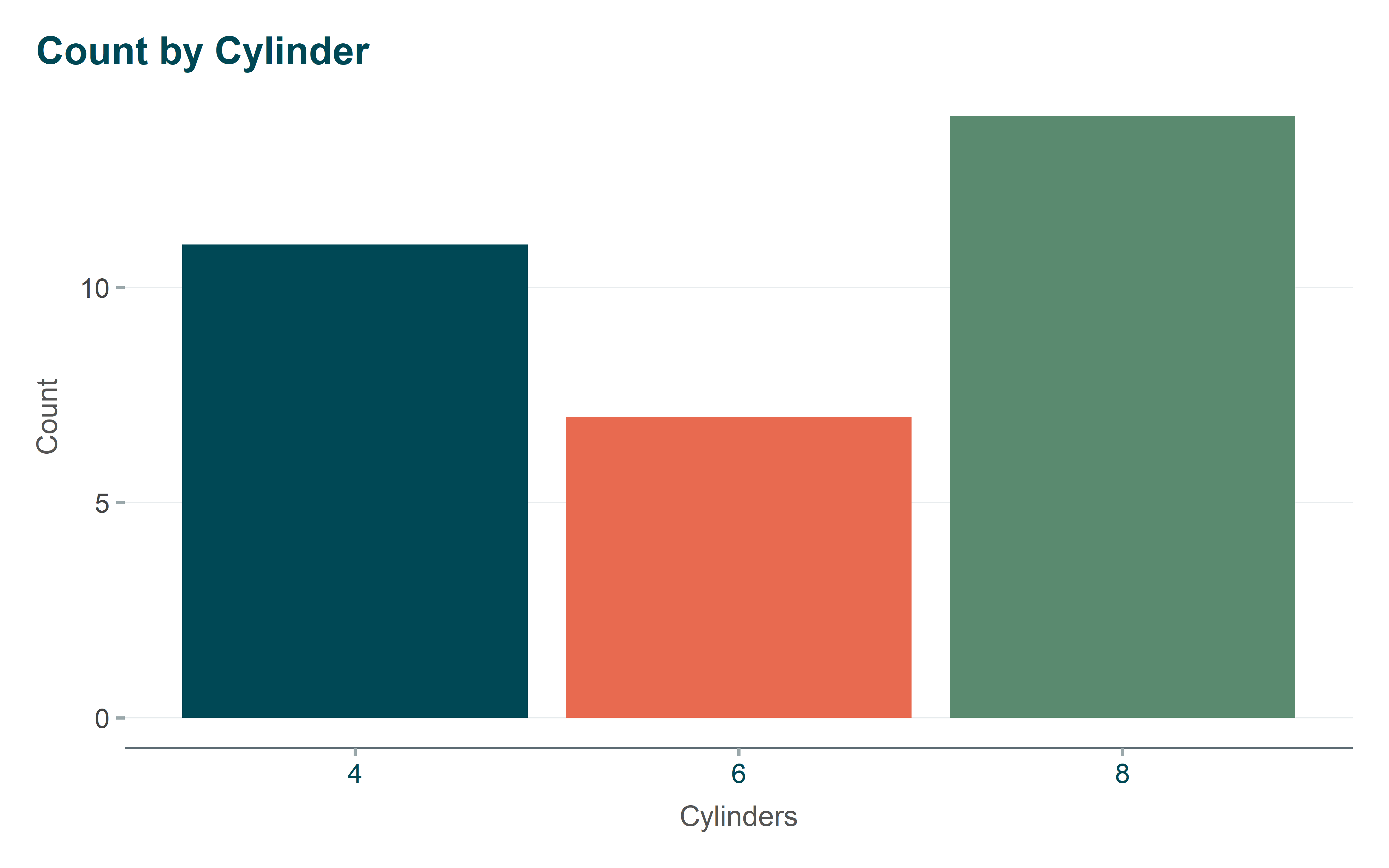
Categorical palettes use visually distinct colors that don’t imply any ordering or magnitude. Each category gets its own easily distinguishable color.

view_cpal_palettes(c("main", "blues", "compare", "binary", "status"))

Usage example:

ggplot(mtcars, aes(x = factor(cyl), fill = factor(cyl))) +
  geom_bar() +
  scale_fill_cpal("main") +  # Use cpal_colors("main", n = 3) for fewer colors
  labs(title = "Count by Cylinder", x = "Cylinders", y = "Count") +
  theme_cpal() +
  theme(legend.position = "none")

---

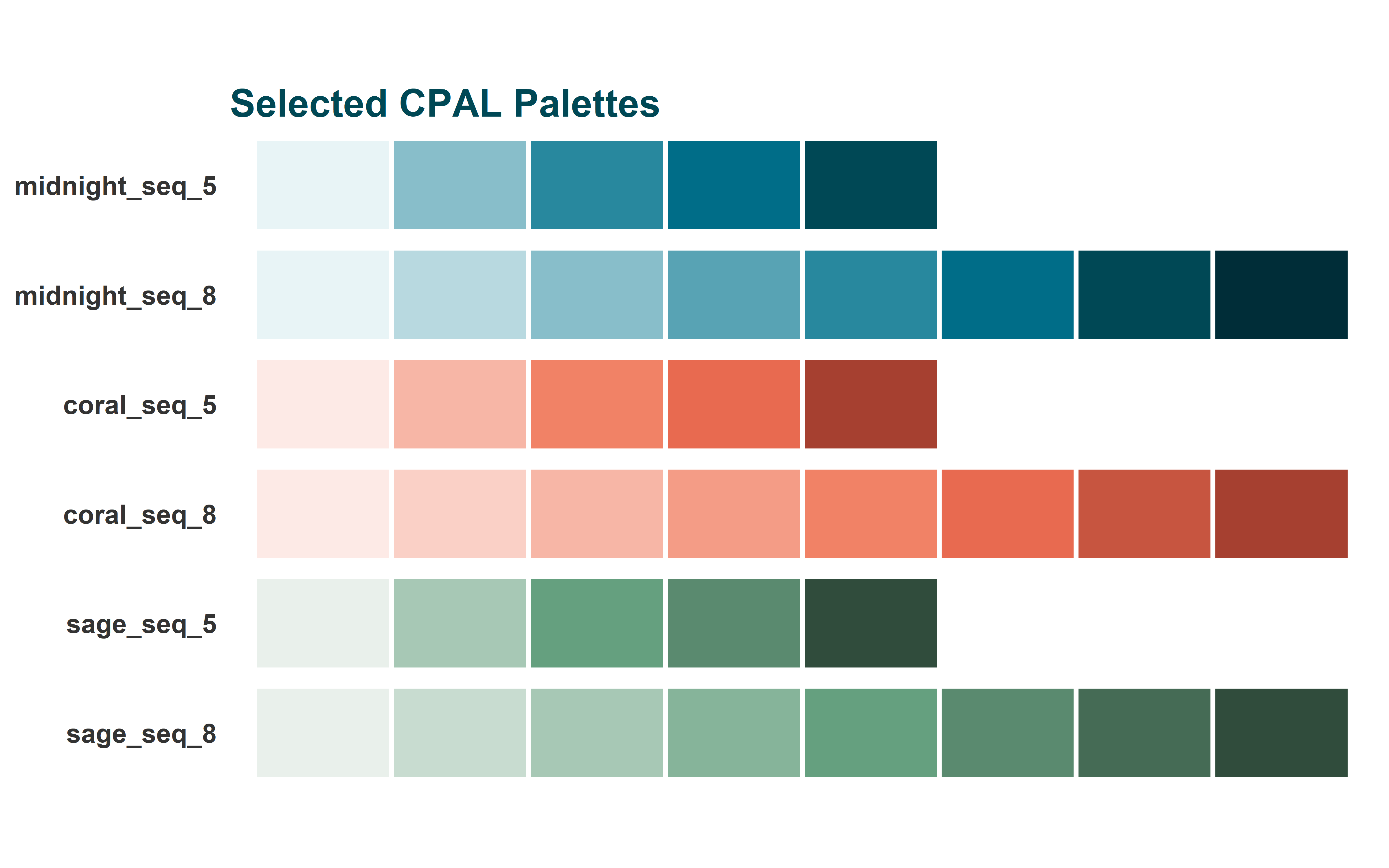
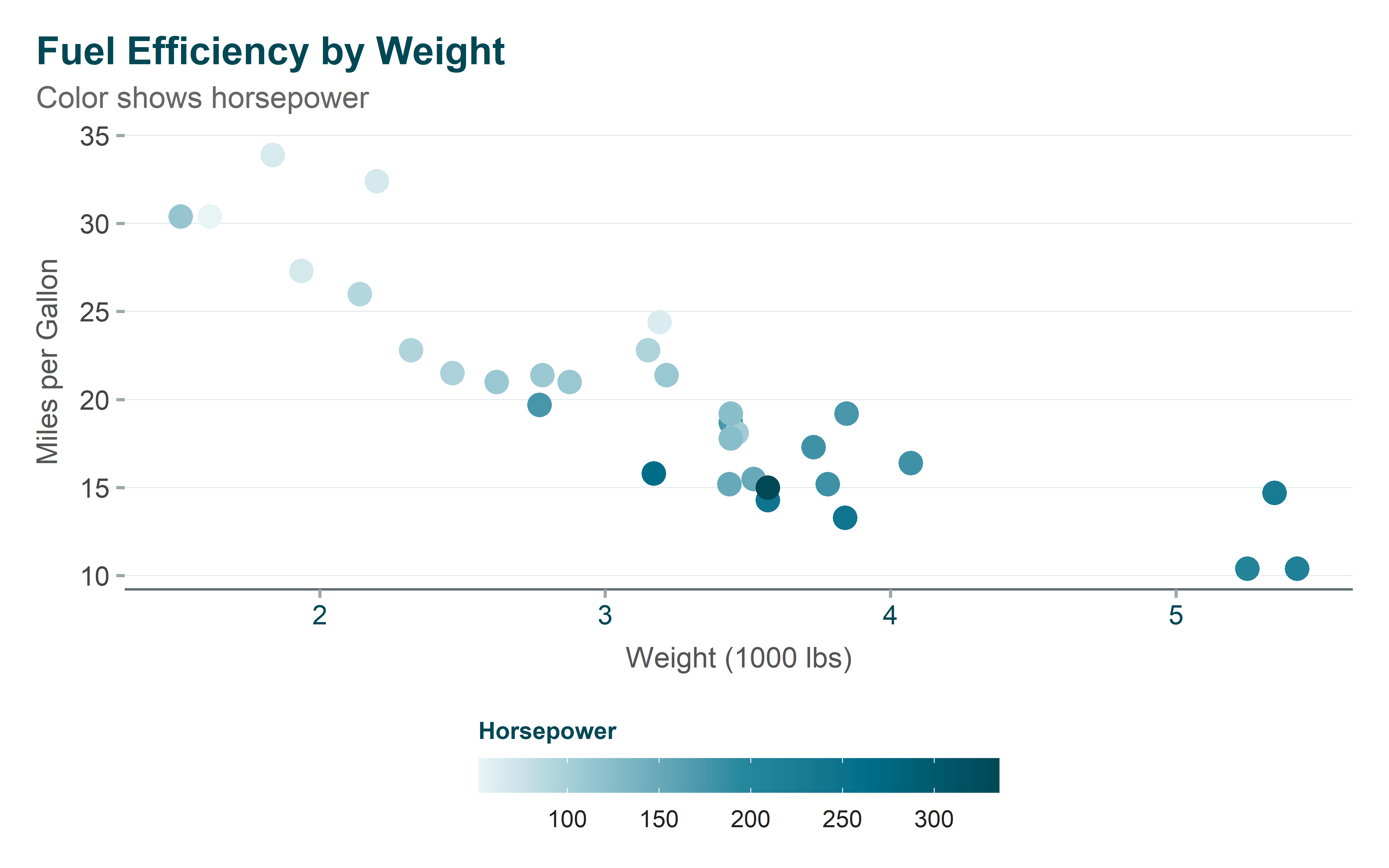
Sequential Palettes

Use for: Continuous or ordered data where values progress from low to high (e.g., population density, income levels, temperature).

Sequential palettes progress from light to dark (or vice versa), allowing readers to intuitively understand that darker colors represent higher values.

view_cpal_palettes(c("midnight_seq_5", "midnight_seq_8", "coral_seq_5", "coral_seq_8", "sage_seq_5", "sage_seq_8"))

Usage example:

ggplot(mtcars, aes(x = wt, y = mpg, color = hp)) +
  geom_point(size = 4) +
  scale_color_cpal_c("midnight_seq_5") +
  labs(
    title = "Fuel Efficiency by Weight",
    subtitle = "Color shows horsepower",
    x = "Weight (1000 lbs)",
    y = "Miles per Gallon",
    color = "Horsepower"
  ) +
  guides(color = guide_colorbar(
    title.position = "top",
    barwidth = 15,
    barheight = 1
  )) +
  theme_cpal()

---

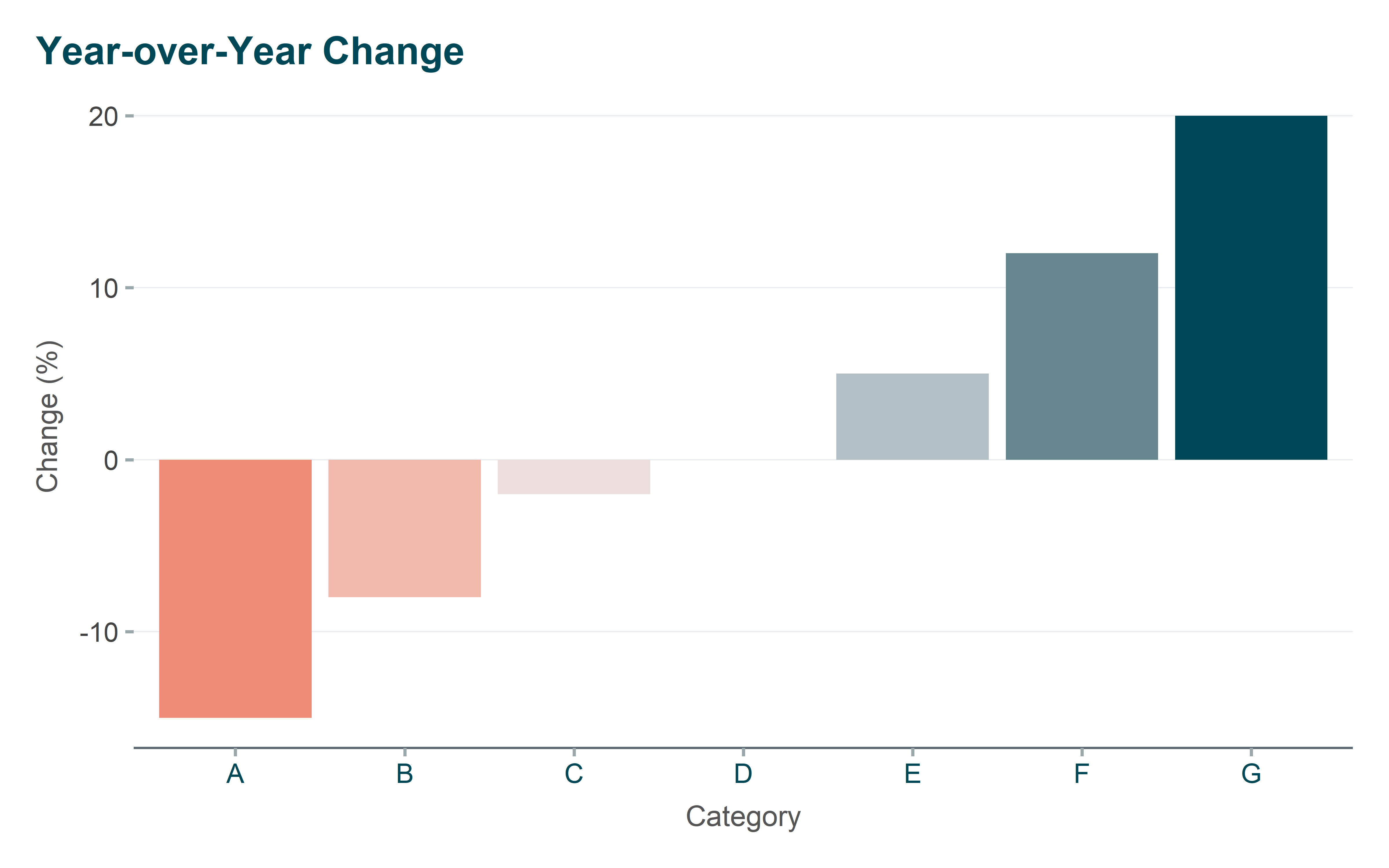
Diverging Palettes

Use for: Data with a meaningful midpoint or neutral value (e.g., year-over-year change, survey responses from negative to positive, deviations from average).

Diverging palettes use two distinct hues that meet at a neutral midpoint, making it easy to see whether values are above or below the center.

view_cpal_palettes(c("coral_midnight_3", "coral_midnight_5", "coral_midnight_7", "coral_midnight_9", "sage_coral_3", "sage_coral_5", "sage_coral_7", "sage_coral_9"))

Usage example:

# Create sample data with positive and negative changes
change_data <- data.frame(
  category = LETTERS[1:7],
  change = c(-15, -8, -2, 0, 5, 12, 20)
)

ggplot(change_data, aes(x = category, y = change, fill = change)) +
  geom_col() +
  scale_fill_gradient2(
    low = "#E86A50",
    mid = "#E8ECEE",
    high = "#004855",
    midpoint = 0
  ) +
  labs(
    title = "Year-over-Year Change",
    x = "Category",
    y = "Change (%)"
  ) +
  theme_cpal() +
  theme(legend.position = "none")

---

ggplot2 Scale Functions

These functions integrate directly with ggplot2, letting you apply CPAL colors using familiar scale_* syntax. They work just like built-in ggplot2 scales but use CPAL’s branded color palettes.

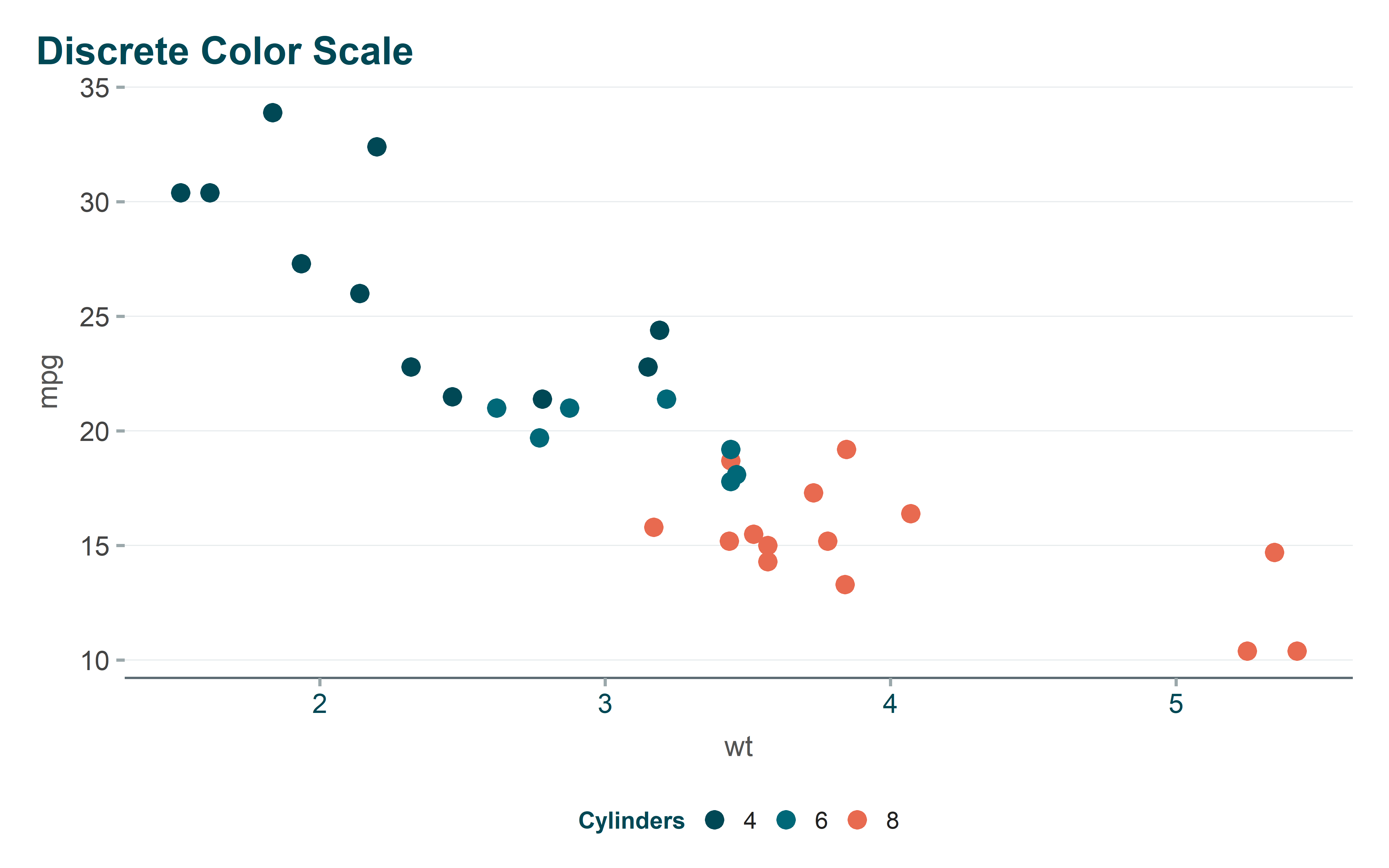
Discrete Scales

Use scale_color_cpal() or scale_fill_cpal() when your data has distinct categories. The function automatically maps each category to a color from your chosen palette.

ggplot(mtcars, aes(x = wt, y = mpg, color = factor(cyl))) +
  geom_point(size = 3) +
  scale_color_cpal("main_3") +
  labs(
    title = "Discrete Color Scale",
    color = "Cylinders"
  ) +
  theme_cpal()

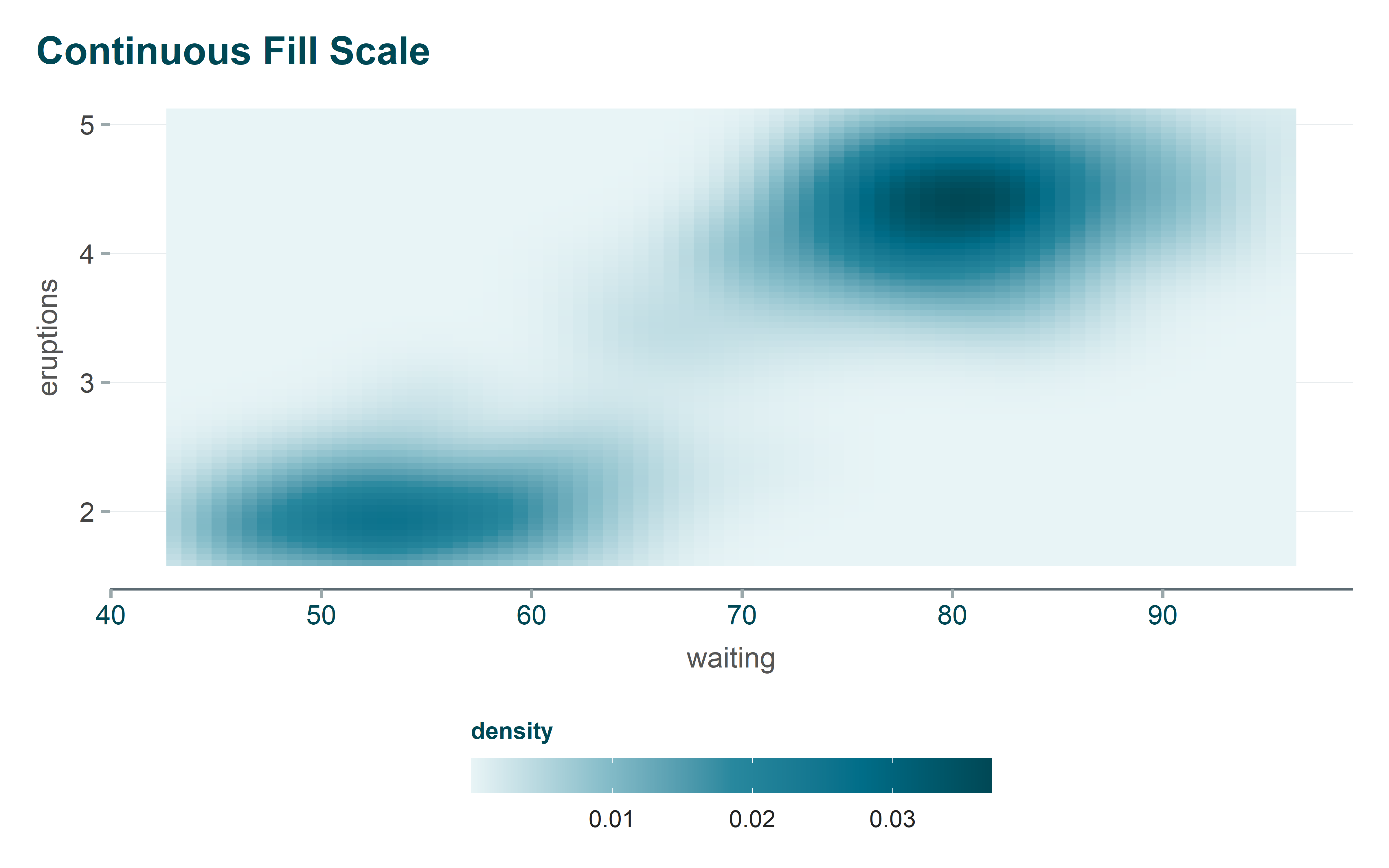
Continuous Scales

Use scale_color_cpal_c() or scale_fill_cpal_c() when your data is numeric and continuous. The function interpolates smoothly across your chosen palette to represent the full range of values.

ggplot(faithfuld, aes(waiting, eruptions, fill = density)) +
  geom_tile() +
  scale_fill_cpal_c("midnight_seq_5") +
  labs(title = "Continuous Fill Scale") +
  guides(fill = guide_colorbar(
    title.position = "top",
    barwidth = 15,
    barheight = 1
  )) +
  theme_cpal()

---

Color Interpolation

Sometimes you need a custom number of colors or a gradient between specific colors that isn’t covered by the standard palettes. These functions let you generate custom color sequences programmatically.

cpal_color_ramp()

Generate a smooth gradient between two CPAL colors. Useful when you need a specific number of steps or want to create a custom sequential palette.

Gradient from coral to midnight

cpal_color_ramp("coral", "midnight", n = 7)

#E86A50

#C16450

#9A5E51

#745952

#4D5353

#264D54

#004855

Using color names from brand.yml

cpal_color_ramp("midnight_1", "midnight", n = 5)

#E8F4F6

#AEC9CD

#749EA5

#39737D

#004855

cpal_color_gradient()

Create a gradient that passes through multiple colors. Perfect for custom diverging palettes or complex color schemes that need to hit specific color waypoints.

Three-color gradient

cpal_color_gradient(c("coral", "neutral", "midnight"), n = 9)

#E86A50

#E88A77

#E8AB9F

#E8CBC6

#E8ECEE

#AEC3C7

#749AA1

#39717B

#004855

---

Color Validation (Accessibility)

Accessibility isn’t just good practice—it’s essential for reaching all audiences. These validation functions help you ensure your color choices meet WCAG (Web Content Accessibility Guidelines) standards, making your R visualizations readable for users with color vision deficiencies.

validate_color_contrast()

Check if two colors meet WCAG contrast requirements. Use this when placing text on colored backgrounds or ensuring data points are distinguishable.

# Check deep_teal on white (should pass AA)
validate_color_contrast("#006878", "#FFFFFF")

# Check with AAA standard (stricter)
validate_color_contrast("#006878", "#FFFFFF", level = "AAA")

# Midnight on white (high contrast)
validate_color_contrast("#004855", "#FFFFFF", level = "AAA")

Click to see output

$foreground
[1] "#006878"

$background
[1] "#FFFFFF"

$contrast_ratio
[1] 6.46

$level
[1] "AA"

$large_text
[1] FALSE

$threshold
[1] 4.5

$passes
[1] TRUE

$recommendation
[1] "Passes WCAG AA (ratio: 6.46:1, required: 4.5:1)"

$foreground
[1] "#006878"

$background
[1] "#FFFFFF"

$contrast_ratio
[1] 6.46

$level
[1] "AAA"

$large_text
[1] FALSE

$threshold
[1] 7

$passes
[1] FALSE

$recommendation
[1] "FAILS WCAG AAA (ratio: 6.46:1, required: 7.0:1). Consider using darker foreground or lighter background."

$foreground
[1] "#004855"

$background
[1] "#FFFFFF"

$contrast_ratio
[1] 10.2

$level
[1] "AAA"

$large_text
[1] FALSE

$threshold
[1] 7

$passes
[1] TRUE

$recommendation
[1] "Passes WCAG AAA (ratio: 10.20:1, required: 7.0:1)"

validate_brand_colors()

Check all CPAL palette colors for accessibility:

validate_brand_colors()

This function prints a detailed report showing which colors pass WCAG AA/AAA standards on white and dark backgrounds.

---

Choosing the Right Palette

Not sure which palette to use? This quick reference helps you match your data type to the appropriate CPAL palette. The goal is to choose colors that help readers understand your data, not just make charts look pretty.

Quick Reference

Data Type	Recommended Palettes
Categories (≤3)	main_3, binary
Categories (4-5)	main_4, main_5
Categories (6-8)	main_6, main
Sequential/Continuous	midnight_seq_5, midnight_seq_6
Diverging (with midpoint)	coral_midnight_5, coral_midnight_7
Binary comparison	binary, compare
Status indicators	status

---

Complete Example

Here’s a complete example showing how CPAL colors, scales, and themes work together in a typical R data visualization workflow. This pattern—data preparation, ggplot2 visualization, CPAL scales, and CPAL theme—is the foundation for all branded CPAL charts.

# Prepare data
car_data <- mtcars |>
  mutate(
    cylinders = factor(cyl),
    efficiency = ifelse(mpg > median(mpg), "High", "Low")
  )

# Create visualization
p1 <- ggplot(car_data, aes(x = hp, y = mpg, color = cylinders, size = wt)) +
  geom_point(alpha = 0.7) +
  scale_color_cpal("main_3") +
  scale_size_continuous(range = c(2, 8)) +
  labs(
    title = "Vehicle Performance Analysis",
    subtitle = "Fuel efficiency by horsepower, colored by cylinder count",
    x = "Horsepower",
    y = "Miles per Gallon",
    color = "Cylinders",
    size = "Weight (1000 lbs)",
    caption = "Source: Motor Trend Car Road Tests (1974)"
  ) +
  theme_cpal()

cpaltemplates::add_cpal_logo(p1)

---

Next Steps

Now that you understand CPAL’s color system, explore these related guides:

• Themes & Styling - Apply themes and save/export plots
• ggplot2 Gallery - See colors in action with example charts
• Highcharter Gallery - CPAL colors in interactive charts